はじめに
現在は機械学習の学習をやっている.
今回はニューラルネットワークのフレームワークであるKeras及びTensorFlowを触ってみることにする.
www.tensorflow.org
上記のチュートリアルを使用し,適宜コメントなどを追加して理解を深めていく.

実装
データの読み込み
#https://www.tensorflow.org/tutorials/keras/classification?hl=ja
# に勉強のために適宜コメントを追加
# TensorFlow と tf.keras のインポート
import tensorflow as tf
from tensorflow import keras
# ヘルパーライブラリのインポート
import numpy as np
import matplotlib.pyplot as plt
print(tf.__version__)
2.6.0
# Fashion-MNIST
# ファッション写真のデータセットをロード
fashion_mnist = keras.datasets.fashion_mnist
(train_images, train_labels), (test_images, test_labels) = fashion_mnist.load_data()
データの可視化
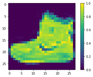
# 訓練データは6万枚,テストデータは1万枚
print(train_images.shape)
print(test_images.shape)

# 1枚目の画像を表示
import matplotlib.pyplot as plt
plt.figure()
plt.imshow(train_images[0])
plt.colorbar()
plt.grid(False)
plt.show()

# 黒が255,白が0,28×28の画像
# 一般的な画像は白が255なので逆
(60000, 28, 28)
(10000, 28, 28)
# ラベルは10種類
print(train_labels.shape)
print(np.unique(train_labels))

# ラベルは[0 1 2 3 4 5 6 7 8 9]のようになっている
# 手動でラベル名を設定しておく
class_names = ['T-shirt/top', 'Trouser', 'Pullover', 'Dress', 'Coat',
               'Sandal', 'Shirt', 'Sneaker', 'Bag', 'Ankle boot']
(60000,)
[0 1 2 3 4 5 6 7 8 9]
# データの正規化(0~1にする)
train_images = train_images / 255.0
test_images = test_images / 255.0
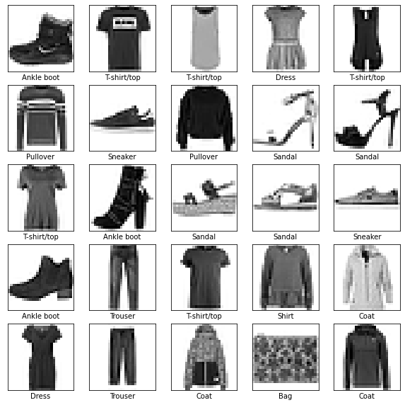
# 訓練データの先頭25枚を表示
plt.figure(figsize=(10,10))
for i in range(25):
    # 5×5に並べて表示
    # subplot(5,5,6)と指定すると,2行1列目部分にプロット
    plt.subplot(5,5,i+1)
    plt.xticks([])
    plt.yticks([])
    plt.grid(False)
    plt.imshow(train_images[i], cmap=plt.cm.binary)
    plt.xlabel(class_names[train_labels[i]])
plt.show()
モデルの構築
# モデルの構築
model = keras.Sequential([
    # 入力層 = 28×28の二次元配列を1次元(28*28=784)に平坦化する
    keras.layers.Flatten(input_shape=(28, 28)),
    # 出力が128個の中間層,活性化関数はReLU
    keras.layers.Dense(128, activation='relu'),
    # 出力が10個の出力層,活性化関数はsoftmax
    keras.layers.Dense(10, activation='softmax')
])
ポンチ絵を描いてみた.
おそらくこんな感じだと思われる.
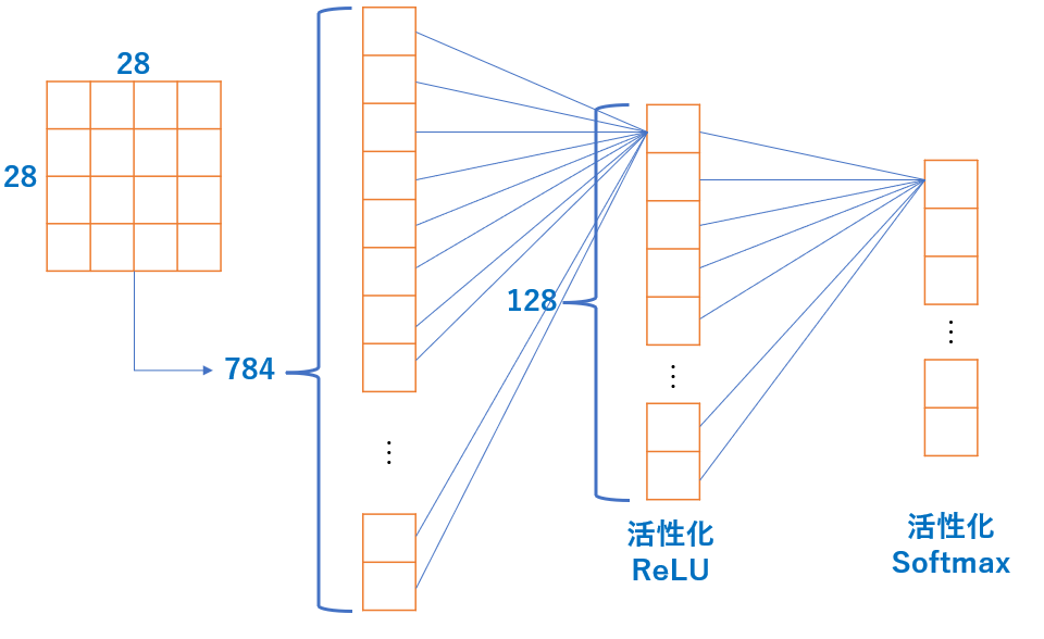
出力層の活性化関数にSoftmax関数を使うのは各出力の総和を1にするため.
各出力を確率として表せる.
例えば['T-shirt/top', 'Trouser', 'Pullover', ...] = [0.7, 0.1, 0.02, ...]という出力になったら,Tシャツの確率が70%であると言える.
# 最適化アルゴリズムはadam
# 誤差関数はクロスエントロピー
# 評価関数は正解率
model.compile(optimizer='adam',
              loss='sparse_categorical_crossentropy',
              metrics=['accuracy'])
最適化アルゴリズムは誤差関数が小さくなるようにネットワークの重みを更新していくアルゴリズム
局所最適解に陥らないように上手い事やる
誤差関数はモデルが出力した結果と正解との差
3値以上の分類にはクロスエントロピーが用いられる
評価関数はモデルの性能(予測精度)を定量的に表すための関数
今回は分類問題の基本的な評価指標であるところのaccuracy(正解率)を使用
keras.io
学習
model.fit(train_images, train_labels, epochs=5)
Epoch 1/5
1875/1875 [==============================] - 2s 742us/step - loss: 0.4980 - accuracy: 0.8238
Epoch 2/5
1875/1875 [==============================] - 1s 698us/step - loss: 0.3736 - accuracy: 0.8659
Epoch 3/5
1875/1875 [==============================] - 1s 731us/step - loss: 0.3346 - accuracy: 0.8796
Epoch 4/5
1875/1875 [==============================] - 1s 699us/step - loss: 0.3123 - accuracy: 0.8866
Epoch 5/5
1875/1875 [==============================] - 1s 698us/step - loss: 0.2928 - accuracy: 0.8919
1エポックあたり1秒くらいで学習が終わった.
test_loss, test_acc = model.evaluate(test_images,  test_labels, verbose=2)

print('\nTest accuracy:', test_acc)
313/313 - 0s - loss: 0.3604 - accuracy: 0.8720
Test accuracy: 0.871999979019165
引数のverboseって何じゃろと検索したところ
www.tensorflow.org
verbose 0 or 1. Verbosity mode. 0 = silent, 1 = progress bar.
とあって0 or 1を取る値とのこと.
何で2を入れてるねんと思ってverbose=1にしたところ以下のようになった.
313/313 [==============================] - 0s 471us/step - loss: 0.3604 - accuracy: 0.8720
Test accuracy: 0.871999979019165
verbose=1だとプログレスバー及びステップごとの計算時間も表示された.
欲しいのは正解率などの指標なので,verbose=2がこの場合は良いっぽい.
予測
# 予測する
predictions = model.predict(test_images)
# 予測結果の1個目を表示
predictions[0]
array([9.9368699e-06, 1.2327422e-07, 1.6504961e-07, 9.8506057e-09,
5.9519666e-06, 3.3276793e-02, 2.7124054e-06, 2.4480930e-01,
3.0131891e-05, 7.2186488e-01], dtype=float32)
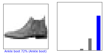
pred_0 = np.argmax(predictions[0])
print(f'予測:{class_names[pred_0]}')
print(f'正解:{class_names[test_labels[0]]}')

# 1枚目の画像を表示
import matplotlib.pyplot as plt
plt.figure()
plt.imshow(test_images[0])
plt.colorbar()
plt.grid(False)
plt.show()
予測:Ankle boot
正解:Ankle boot
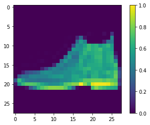
となり,1個目は正解した.
predictions[0].sum()
# = 1.0
なお,結果の合計値を計算してみると確かに1.0になっており,Softmax関数による確率表現となっている.
def plot_image(i, predictions_array, true_label, img):
    predictions_array, true_label, img = predictions_array[i], true_label[i], img[i]
    plt.grid(False)
    plt.xticks([])
    plt.yticks([])

    plt.imshow(img, cmap=plt.cm.binary)

    predicted_label = np.argmax(predictions_array)
    if predicted_label == true_label:
        color = 'blue'
    else:
        color = 'red'

    plt.xlabel("{} {:2.0f}% ({})".format(class_names[predicted_label],
                                    100*np.max(predictions_array),
                                    class_names[true_label]),
                                    color=color)

def plot_value_array(i, predictions_array, true_label):
    predictions_array, true_label = predictions_array[i], true_label[i]
    plt.grid(False)
    plt.xticks([])
    plt.yticks([])
    thisplot = plt.bar(range(10), predictions_array, color="#777777")
    plt.ylim([0, 1])
    predicted_label = np.argmax(predictions_array)

    thisplot[predicted_label].set_color('red')
    thisplot[true_label].set_color('blue')
結果を表示する関数を実装.
i = 0
plt.figure(figsize=(6,3))
plt.subplot(1,2,1)
plot_image(i, predictions, test_labels, test_images)
plt.subplot(1,2,2)
plot_value_array(i, predictions,  test_labels)
plt.show()
i = 12
plt.figure(figsize=(6,3))
plt.subplot(1,2,1)
plot_image(i, predictions, test_labels, test_images)
plt.subplot(1,2,2)
plot_value_array(i, predictions,  test_labels)
plt.show()
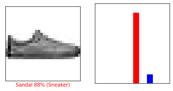
88%の確率でサンダルです!っつって間違ってしまっている.
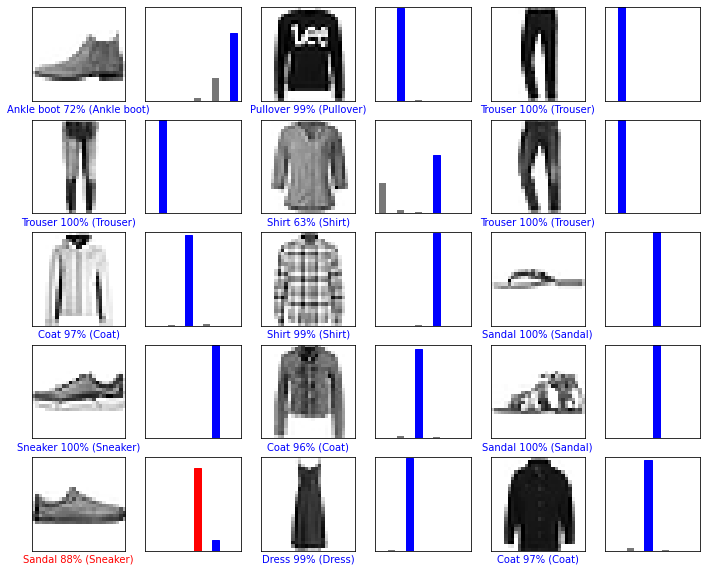
# X個のテスト画像,予測されたラベル,正解ラベルを表示します.
# 正しい予測は青で,間違った予測は赤で表示しています.
num_rows = 5
num_cols = 3
num_images = num_rows*num_cols
plt.figure(figsize=(2*2*num_cols, 2*num_rows))
for i in range(num_images):
  plt.subplot(num_rows, 2*num_cols, 2*i+1)
  plot_image(i, predictions, test_labels, test_images)
  plt.subplot(num_rows, 2*num_cols, 2*i+2)
  plot_value_array(i, predictions, test_labels)
plt.show()
まとめ
今回はKeras及びTensorFlowのチュートリアルを進めた.
中間層が1つしか無いが,正解率87%という良い結果を得られた.
Kerasのおかげで大分実装が簡単になっている.
層とか評価関数を引数として指定するだけだからね.
ニューラルネットワークの実装はKerasがやってくれるため,
私の方ではデータや結果の可視化をしっかりとやっていく必要があると感じた.
また,スニーカーの画像を自信満々(88%)にサンダルと言って間違うということもあり,そこはせめて迷って欲しかった.
(サンダル60%,スニーカー40%の確率で判定した,とか)
